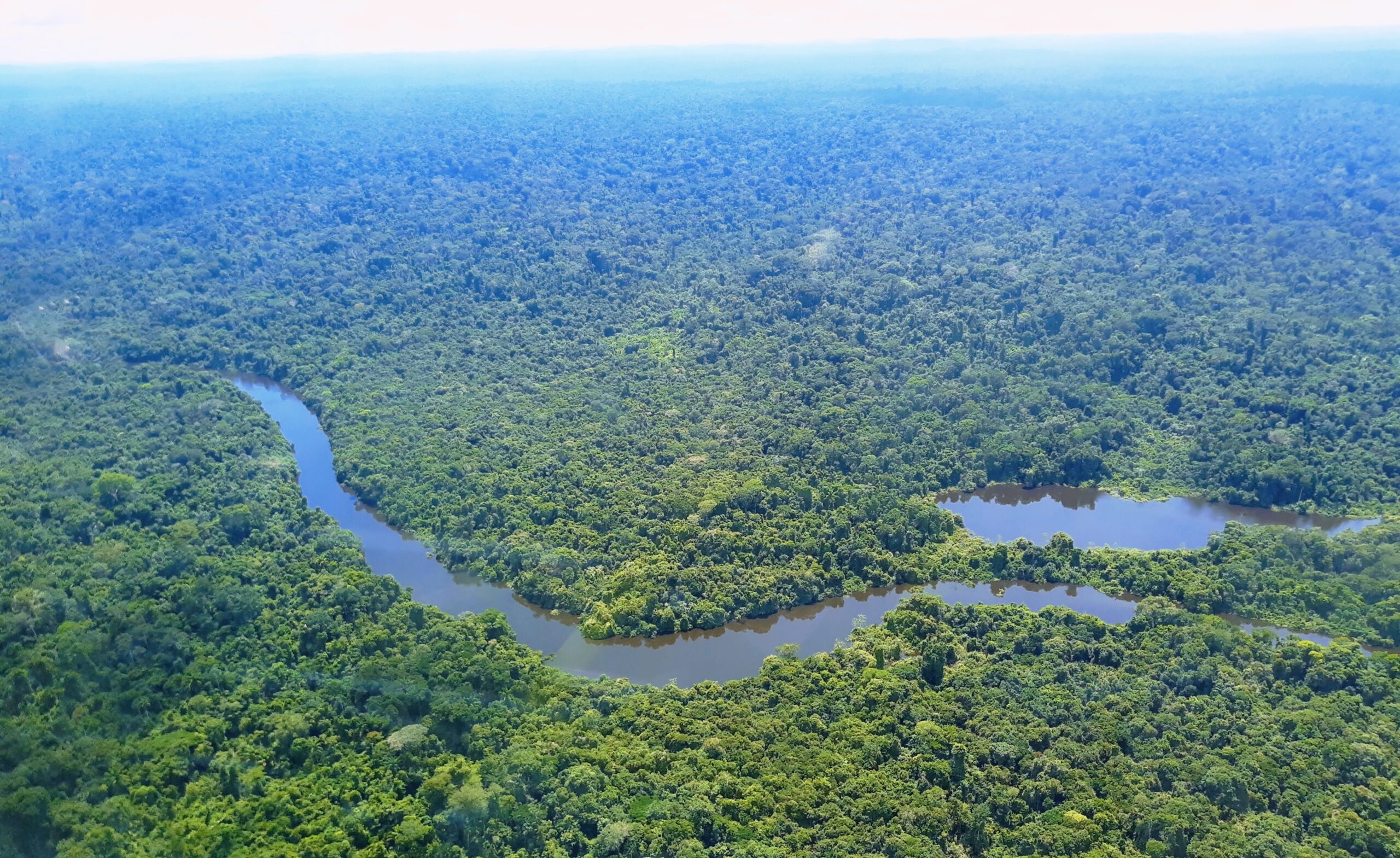
Small data, big problems. That’s the reality for geospatial machine learning. Forget terabytes of text. Here, we’re talking about painstakingly collected GPS points, each one costing more than your latest graphics card. Building AI models that can map the planet, or at least significant chunks of it, is often hampered by this infuriatingly expensive reality of fieldwork.
And when I say expensive, I mean expensive. A single forest inventory plot in, say, the Amazon rainforest can set you back the price of a decent ML workstation. This isn’t a hypothetical. It’s the daily grind for folks in environmental science, forestry, and remote sensing. They’ve got oceans of satellite imagery, but precious little ground truth to train their AI models on.
The Tyranny of Expensive Pixels
Think about it. You’ve got a massive area. You’ve got mountains of satellite data, topographic models, maybe even some spectral indices. Then you have your handful of reference points. Maybe 100, maybe 200. Sounds like a lot, right? Wrong. In the wild, spatially correlated world of environmental data, that number can vanish faster than free donuts in the breakroom. Environmental heterogeneity, or the ‘messiness’ of the real world, starts chewing up your precious samples, leaving you with more questions than answers.
This isn’t just an academic exercise. It’s about creating maps that matter, maps that guide conservation efforts, resource management, or disaster response. And those maps are useless if they’re built on shaky, data-starved models. The whole exercise becomes a frustrating dance between what’s technically possible and what’s financially feasible.
The problem comes up frequently in environmental, forestry, and remote sensing applications, but it isn’t exclusive to those contexts. The logic applies to any continuous spatial variable where images, mosaics, and data cubes exist in abundance, but field labels are expensive, rare, and imperfect.
Squeeze Every Drop From Your Data
So, what’s the workaround when your budget looks more like a shoestring than a king’s ransom? The article here wisely steers clear of the ‘throw more tech at it’ approach. Instead, it champions the unglamorous but effective strategy of extracting more juice from each existing data point. This means smart feature engineering and data integration. Don’t just feed your model a single spectral band. Combine optical data with LiDAR for structure, throw in some topographic variables, and — if it’s relevant — that temporal context, like flood patterns or seasonal droughts. The goal isn’t to stuff your feature matrix until it groans, but to create a lean, mean, informative set of variables. Think of it as giving your model a more detailed dossier on each location, rather than just a name and an address.
Models That Don’t Overfit Their Patrons
When data is thin on the ground, model selection becomes less about chasing state-of-the-art benchmarks and more about avoiding a catastrophic case of memorization. Highly flexible models, the ones that can bend and contort themselves to fit every nook and cranny of your training data, are the enemy here. They’ll happily learn spurious correlations and random noise, mistaking them for genuine signals. That’s how you end up with a model that looks brilliant on paper but generates wildly inaccurate maps in the real world.
Tree-based algorithms, like Random Forest or gradient boosting (XGBoost, anyone?), often hit that sweet spot. They’re not overly complex, they offer built-in regularization, and they can handle non-linearities without completely losing their minds. The trade-off is constant: more depth means more detail but also more risk of memorizing noise. The objective isn’t peak performance on a single data split; it’s about finding a configuration that remains sensible when the model ventures beyond the familiar territory of your training samples.
Validation That Doesn’t Lie
Here’s where things get really dicey. The fastest way to fool yourself in geospatial ML is to use standard random cross-validation. Why? Because spatially autocorrelated data means nearby points share environments, histories, and even sensor artifacts. Splitting those points randomly between training and testing sets gives you artificially inflated performance metrics. It looks like generalization, but it’s really just interpolation within a familiar neighborhood. The model hasn’t learned anything new; it’s just memorized the local décor.
Spatial validation is therefore not optional; it’s mandatory. Whether it’s block cross-validation, leave-one-out for small regions, or more advanced techniques, the key is to ensure your test data represents truly novel spatial contexts. This prevents the embarrassing situation where your model aces the internal tests but fails spectacularly when deployed in the wild, spitting out maps that are fundamentally divorced from reality.
Communicating Uncertainty: The Human Element
And finally, there’s the human factor. When you’re dealing with limited data, the output isn’t just a map; it’s a map with caveats. Being transparent about the uncertainty baked into your model’s predictions is paramount. This means clearly communicating where the model is likely to be accurate and, more importantly, where it’s likely to be wrong. Visualizing uncertainty—showing not just the predicted value but a range of plausible values—is critical. It manages expectations and prevents misinformed decisions based on an overconfident, but ultimately unreliable, AI prediction.
This whole approach to small data geospatial ML feels like a much-needed dose of pragmatism in a field often chasing the latest, most computationally intensive model. It’s a reminder that sometimes, the smartest path forward involves working harder with what you have, not just wishing for more.
🧬 Related Insights
- Read more: C# 15 Union Types: The End of Tedious Type Checks in .NET 11
- Read more: Amazon Quick Gets Observability: What It Means for Your AI ROI
Frequently Asked Questions
What does ‘small data’ mean for geospatial ML?
It means having a limited number of ground-truth locations or samples for training. These samples are costly and time-consuming to collect, making large datasets infeasible.
Why is random cross-validation bad for geospatial data?
Geospatial data is often spatially autocorrelated, meaning nearby points share similar characteristics. Random splits can put similar training and testing points together, leading to inflated performance metrics that don’t reflect real-world generalization.
How can I improve my geospatial ML models with limited data?
Focus on extracting more information from each sample through feature engineering, choosing simpler models that regularize well, and implementing strong spatial validation techniques. Clearly communicating model uncertainty is also crucial.